机器学习(12)之决策树总结与python实践(~附源码链接~)

微信公众号
关键字全网搜索最新排名
【机器学习算法】:排名第一
【机器学习】:排名第二
【Python】:排名第三
【算法】:排名第四
前言
在(机器学习(9)之ID3算法详解及python实现)中讲到了ID3算法,在(机器学习(11)之C4.5详解与Python实现(从解决ID3不足的视角))中论述了ID3算法的改进版C4.5算法。对于C4.5算法,也提到了它的不足,比如模型是用较为复杂的熵来度量,使用了相对较为复杂的多叉树,只能处理分类不能处理回归等。对于这些问题, CART算法大部分做了改进。由于CART算法可以做回归,也可以做分类,本文以CART作为分类树来论述。
最优特征选择方法
在ID3算法中使用了信息增益来选择特征,信息增益大的优先选择。在C4.5算法中采用了信息增益比来选择特征,以减少信息增益容易选择特征值多的特征的问题。但是无论ID3还是C4.5,都是基于信息论的熵模型的,这里面会涉及大量的对数运算。能不能简化模型同时也不至于完全丢失熵模型的优点呢?有!CART分类树算法使用基尼系数来代替信息增益比,基尼系数代表了模型的不纯度,基尼系数越小,则不纯度越低,特征越好。这和信息增益(比)是相反的。
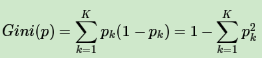
在分类问题中,假设有K个类别,第k个类别的概率为pk, 则基尼系数的表达式为:
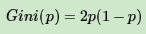
若是二类分类问题,计算就更简单了,如果属于第一个样本输出的概率是p,则基尼系数的表达式为:
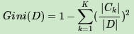
对于给定样本D,假设有K个类别, 第k个类别的数量为Ck,则样本D的基尼系数表达式为:
特别的,对于样本D,如果根据特征A的某个值a,把D分成D1和D2两部分,则在特征A的条件下,D的基尼系数表达式为:

为了进一步简化,CART分类树算法每次仅仅对某个特征的值进行二分,而不是多分,这样CART分类树算法建立起来的是二叉树,而不是多叉树。这样一可以进一步简化基尼系数的计算,二可以建立一个更加优雅的二叉树模型。
连续特征的处理
对于CART分类树连续值的处理问题,其思想和C4.5是相同的,都是将连续的特征离散化。唯一的区别在于在选择划分点时的度量方式不同,C4.5使用的是信息增益,则CART分类树使用的是基尼系数。
具体的思路如下(与C4.5一致),比如m个样本的连续特征A有m个,从小到大排列为a1,a2,...,am,则CART算法取相邻两样本值的中位数,一共取得m-1个划分点,其中第i个划分点表示Ti表示为:Ti=ai+ai+12。对于这m-1个点,分别计算以该点作为二元分类点时的基尼系数。选择基尼系数最小的点作为该连续特征的二元离散分类点。
对于CART分类树离散值的处理问题,采用的思路是不停的二分离散特征。回忆下ID3或者C4.5,如果某个特征A被选取建立决策树节点,如果它有A1,A2,A3三种类别,我们会在决策树上一下建立一个三叉的节点。这样导致决策树是多叉树。但是CART分类树使用的方法不同,他采用的是不停的二分,还是这个例子,CART分类树会考虑把A分成和{A1}和{A2,A3}, 和{A2}和{A1,A3}, 和{A3}和{A1,A2}三种情况,找到基尼系数最小的组合,比如和{A2}和{A1,A3},然后建立二叉树节点,一个节点是A2对应的样本,另一个节点是{A1,A3}对应的节点。同时,由于这次没有把特征A的取值完全分开,后面我们还有机会在子节点继续选择到特征A来划分A1和A3。这和ID3或者C4.5不同,在ID3或者C4.5的一棵子树中,离散特征只会参与一次节点的建立。
CART建树流程
算法输入是训练集D,基尼系数的阈值,样本个数阈值。
算法输出是决策树T。
1) 对于当前节点的数据集为D,如果样本个数小于阈值或者没有特征,则返回决策子树,当前节点停止递归。
2) 计算样本集D的基尼系数,如果基尼系数小于阈值,则返回决策树子树,当前节点停止递归。
3) 计算当前节点现有的各个特征的各个特征值对数据集D的基尼系数,对于离散值和连续值的处理方法和基尼系数的计算见上一节。
4) 在计算出来的各个特征的各个特征值对数据集D的基尼系数中,选择基尼系数最小的特征A和对应的特征值a。根据这个最优特征和最优特征值,把数据集划分成两部分D1和D2,同时建立当前节点的左右节点,做节点的数据集D为D1,右节点的数据集D为D2.
5) 对左右的子节点递归的调用1-4步,生成决策树。
剪枝
第一步是从原始决策树生成各种剪枝效果的决策树;
第二步是用交叉验证来检验剪枝后的预测能力,选择泛化预测能力最好的剪枝后的数作为最终的CART树。
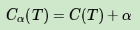
在剪枝的过程中,对于任意的一刻子树T,其损失函数为:
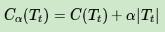
其中,α为正则化参数,C(Tt)为训练数据的预测误差,分类树是用基尼系数度量,回归树是均方差度量。|Tt|是子树T的叶子节点的数量。
当α=0时,即没有正则化,原始的生成的CART树即为最优子树。当α=∞时,即正则化强度达到最大,此时由原始的生成的CART树的根节点组成的单节点树为最优子树。一般来说,α越大,则剪枝剪的越厉害,生成的最优子树相比原生决策树就越偏小。对于固定的α,一定存在使损失函数Cα(T)最小的唯一子树。
对于位于节点t的任意一颗子树Tt,如果没有剪枝,它的损失是上面的那个公式。如果将其剪掉,仅仅保留根节点,则损失是
如果满足下式:
Tt和T有相同的损失函数,但是T节点更少,因此可以对子树Tt进行剪枝,也就是将它的子节点全部剪掉,变为一个叶子节点T。
剪枝流程
输入是CART树建立算法得到的原始决策树T。
输出是最优决策子树Tα。
算法过程如下:
1)初始化αmin=∞, 最优子树集合ω={T}。
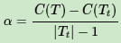
2)从叶子节点开始自下而上计算各内部节点t的训练误差损失函数Cα(Tt)(回归树为均方差,分类树为基尼系数), 叶子节点数|Tt|,以及正则化阈值α=min{C(T)−C(Tt)|Tt|−1,αmin}, 更新αmin=α
3) 得到所有节点的α值的集合M。
4)从M中选择最大的值αk,自上而下的访问子树t的内部节点,如果(C(T)−C(Tt))/(|Tt|−1)≤αk时,进行剪枝。并决定叶节点t的值。如果是分类树,则是概率最高的类别,如果是回归树,则是所有样本输出的均值。这样得到αk对应的最优子树Tk
5)最优子树集合ω=ω∪Tk, M=M−{αk}。
6) 如果M不为空,则回到步骤4。否则就已经得到了所有的可选最优子树集合ω.
7) 采用交叉验证在ω选择最优子树
三类算法对比
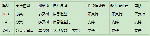
优点
1)简单直观,生成的决策树很直观。
2)基本不需要预处理,不需要提前归一化,处理缺失值。
3)使用决策树预测的代价是O(log2m)。 m为样本数。
4)既可以处理离散值也可以处理连续值。很多算法只是专注于离散值或者连续值。
5)可以处理多维度输出的分类问题。
6)相比于神经网络之类的黑盒分类模型,决策树在逻辑上可以得到很好的解释
7)可以交叉验证的剪枝来选择模型,从而提高泛化能力。
8) 对于异常点的容错能力好,健壮性高。
缺点
1)决策树算法非常容易过拟合,导致泛化能力不强。可以通过设置节点最少样本数量和限制决策树深度来改进。
2)决策树会因为样本发生一点点的改动,就会导致树结构的剧烈改变。这个可以通过集成学习之类的方法解决。
3)寻找最优的决策树是一个NP难的问题,我们一般是通过启发式方法,容易陷入局部最优。可以通过集成学习之类的方法来改善。
4)有些比较复杂的关系,决策树很难学习,比如异或。这个就没有办法了,一般这种关系可以换神经网络分类方法来解决。
5)如果某些特征的样本比例过大,生成决策树容易偏向于这些特征。这个可以通过调节样本权重来改善。
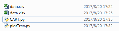
CART实战
数据参照 《机器学习-周志华》 一书中的决策树一章。
代码则参照《机器学习实战》一书的内容,并做了一些修改。
源码下载方式
- 添加微信交流群(加我微信:guodongwe1991,备注姓名-单位-研究方向)
- 后台回复关键词:170821

其中,前11个数据用作训练集(1, 2, 3, 6, 7, 10, 14, 15, 16, 17, 4),后6个数据用作测试集(5,8,9,11,12,13)
CART.py(代码233行)
# -*- coding: utf-8 -*-
from numpy import *
import numpy as np
import pandas as pd
from math import log
import operator
#计算数据集的基尼指数
def calcGini(dataSet):
numEntries=len(dataSet)
labelCounts={}
#给所有可能分类创建字典
for featVec in dataSet:
currentLabel=featVec[-1]
if currentLabel not in labelCounts.keys():
labelCounts[currentLabel]=0
labelCounts[currentLabel]+=1
Gini=1.0
#以2为底数计算香农熵
for key in labelCounts:
prob = float(labelCounts[key])/numEntries
Gini-=prob*prob
return Gini
#对离散变量划分数据集,取出该特征取值为value的所有样本
def splitDataSet(dataSet,axis,value):
retDataSet=[]
for featVec in dataSet:
if featVec[axis]==value:
reducedFeatVec=featVec[:axis]
reducedFeatVec.extend(featVec[axis+1:])
retDataSet.append(reducedFeatVec)
return retDataSet
#对连续变量划分数据集,direction规定划分的方向,
#决定是划分出小于value的数据样本还是大于value的数据样本集
def splitContinuousDataSet(dataSet,axis,value,direction):
retDataSet=[]
for featVec in dataSet:
if direction==0:
if featVec[axis]>value:
reducedFeatVec=featVec[:axis]
reducedFeatVec.extend(featVec[axis+1:])
retDataSet.append(reducedFeatVec)
else:
if featVec[axis]<=value:
reducedFeatVec=featVec[:axis]
reducedFeatVec.extend(featVec[axis+1:])
retDataSet.append(reducedFeatVec)
return retDataSet
#选择最好的数据集划分方式
def chooseBestFeatureToSplit(dataSet,labels):
numFeatures=len(dataSet[0])-1
bestGiniIndex=100000.0
bestFeature=-1
bestSplitDict={}
for i in range(numFeatures):
featList=[example[i] for example in dataSet]
#对连续型特征进行处理
if type(featList[0]).__name__=='float' or type(featList[0]).__name__=='int':
#产生n-1个候选划分点
sortfeatList=sorted(featList)
splitList=[]
for j in range(len(sortfeatList)-1):
splitList.append((sortfeatList[j]+sortfeatList[j+1])/2.0)
bestSplitGini=10000
slen=len(splitList)
#求用第j个候选划分点划分时,得到的信息熵,并记录最佳划分点
for j in range(slen):
value=splitList[j]
newGiniIndex=0.0
subDataSet0=splitContinuousDataSet(dataSet,i,value,0)
subDataSet1=splitContinuousDataSet(dataSet,i,value,1)
prob0=len(subDataSet0)/float(len(dataSet))
newGiniIndex+=prob0*calcGini(subDataSet0)
prob1=len(subDataSet1)/float(len(dataSet))
newGiniIndex+=prob1*calcGini(subDataSet1)
if newGiniIndex<bestSplitGini:
bestSplitGini=newGiniIndex
bestSplit=j
#用字典记录当前特征的最佳划分点
bestSplitDict[labels[i]]=splitList[bestSplit]
GiniIndex=bestSplitGini
#对离散型特征进行处理
else:
uniqueVals=set(featList)
newGiniIndex=0.0
#计算该特征下每种划分的信息熵
for value in uniqueVals:
subDataSet=splitDataSet(dataSet,i,value)
prob=len(subDataSet)/float(len(dataSet))
newGiniIndex+=prob*calcGini(subDataSet)
GiniIndex=newGiniIndex
if GiniIndex<bestGiniIndex:
bestGiniIndex=GiniIndex
bestFeature=i
#若当前节点的最佳划分特征为连续特征,则将其以之前记录的划分点为界进行二值化处理
#即是否小于等于bestSplitValue
if type(dataSet[0][bestFeature]).__name__=='float' or type(dataSet[0][bestFeature]).__name__=='int':
bestSplitValue=bestSplitDict[labels[bestFeature]]
labels[bestFeature]=labels[bestFeature]+'<='+str(bestSplitValue)
for i in range(shape(dataSet)[0]):
if dataSet[i][bestFeature]<=bestSplitValue:
dataSet[i][bestFeature]=1
else:
dataSet[i][bestFeature]=0
return bestFeature
#特征若已经划分完,节点下的样本还没有统一取值,则需要进行投票
def majorityCnt(classList):
classCount={}
for vote in classList:
if vote not in classCount.keys():
classCount[vote]=0
classCount[vote]+=1
return max(classCount)
#主程序,递归产生决策树
def createTree(dataSet,labels,data_full,labels_full):
classList=[example[-1] for example in dataSet]
if classList.count(classList[0])==len(classList):
return classList[0]
if len(dataSet[0])==1:
return majorityCnt(classList)
bestFeat=chooseBestFeatureToSplit(dataSet,labels)
bestFeatLabel=labels[bestFeat]
myTree={bestFeatLabel:{}}
featValues=[example[bestFeat] for example in dataSet]
uniqueVals=set(featValues)
if type(dataSet[0][bestFeat]).__name__=='str':
currentlabel=labels_full.index(labels[bestFeat])
featValuesFull=[example[currentlabel] for example in data_full]
uniqueValsFull=set(featValuesFull)
del(labels[bestFeat])
#针对bestFeat的每个取值,划分出一个子树。
for value in uniqueVals:
subLabels=labels[:]
if type(dataSet[0][bestFeat]).__name__=='str':
uniqueValsFull.remove(value)
myTree[bestFeatLabel][value]=createTree(splitDataSet\
(dataSet,bestFeat,value),subLabels,data_full,labels_full)
if type(dataSet[0][bestFeat]).__name__=='str':
for value in uniqueValsFull:
myTree[bestFeatLabel][value]=majorityCnt(classList)
return myTree
#由于在Tree中,连续值特征的名称以及改为了 feature<=value的形式
#因此对于这类特征,需要利用正则表达式进行分割,获得特征名以及分割阈值
def classify(inputTree,featLabels,testVec):
firstStr=inputTree.keys()[0]
if '<=' in firstStr:
featvalue=float(re.compile("(<=.+)").search(firstStr).group()[2:])
featkey=re.compile("(.+<=)").search(firstStr).group()[:-2]
secondDict=inputTree[firstStr]
featIndex=featLabels.index(featkey)
if testVec[featIndex]<=featvalue:
judge=1
else:
judge=0
for key in secondDict.keys():
if judge==int(key):
if type(secondDict[key]).__name__=='dict':
classLabel=classify(secondDict[key],featLabels,testVec)
else:
classLabel=secondDict[key]
else:
secondDict=inputTree[firstStr]
featIndex=featLabels.index(firstStr)
for key in secondDict.keys():
if testVec[featIndex]==key:
if type(secondDict[key]).__name__=='dict':
classLabel=classify(secondDict[key],featLabels,testVec)
else:
classLabel=secondDict[key]
return classLabel
#测试决策树正确率
def testing(myTree,data_test,labels):
error=0.0
for i in range(len(data_test)):
if classify(myTree,labels,data_test[i])!=data_test[i][-1]:
error+=1
#print 'myTree %d' %error
return float(error)
#测试投票节点正确率
def testingMajor(major,data_test):
error=0.0
for i in range(len(data_test)):
if major!=data_test[i][-1]:
error+=1
#print 'major %d' %error
return float(error)
#后剪枝
def postPruningTree(inputTree,dataSet,data_test,labels):
firstStr=inputTree.keys()[0]
secondDict=inputTree[firstStr]
classList=[example[-1] for example in dataSet]
featkey=copy.deepcopy(firstStr)
if '<=' in firstStr:
featkey=re.compile("(.+<=)").search(firstStr).group()[:-2]
featvalue=float(re.compile("(<=.+)").search(firstStr).group()[2:])
labelIndex=labels.index(featkey)
temp_labels=copy.deepcopy(labels)
del(labels[labelIndex])
for key in secondDict.keys():
if type(secondDict[key]).__name__=='dict':
if type(dataSet[0][labelIndex]).__name__=='str':
inputTree[firstStr][key]=postPruningTree(secondDict[key],\
splitDataSet(dataSet,labelIndex,key),splitDataSet(data_test,labelIndex,key),copy.deepcopy(labels))
else:
inputTree[firstStr][key]=postPruningTree(secondDict[key],\
splitContinuousDataSet(dataSet,labelIndex,featvalue,key),\
splitContinuousDataSet(data_test,labelIndex,featvalue,key),\
copy.deepcopy(labels))
if testing(inputTree,data_test,temp_labels)<=testingMajor(majorityCnt(classList),data_test):
return inputTree
return majorityCnt(classList)
df=pd.read_csv('data.csv')
data=df.values[:11,1:].tolist()
data_full=data[:]
labels=df.columns.values[1:-1].tolist()
labels_full=labels[:]
myTree=createTree(data,labels,data_full,labels_full)
data=df.values[:11,1:].tolist()
data_test=df.values[11:,1:].tolist()
labels=df.columns.values[1:-1].tolist()
myTree=postPruningTree(myTree,data,data_test,labels)
import plotTree
plotTree.createPlot(myTree)
plotTree.py(代码72行)
import matplotlib.pyplot as plt
decisionNode=dict(boxstyle="sawtooth",fc="0.8")
leafNode=dict(boxstyle="round4",fc="0.8")
arrow_args=dict(arrowstyle="<-")
#计算树的叶子节点数量
def getNumLeafs(myTree):
numLeafs=0
firstStr=myTree.keys()[0]
secondDict=myTree[firstStr]
for key in secondDict.keys():
if type(secondDict[key]).__name__=='dict':
numLeafs+=getNumLeafs(secondDict[key])
else: numLeafs+=1
return numLeafs
#计算树的最大深度
def getTreeDepth(myTree):
maxDepth=0
firstStr=myTree.keys()[0]
secondDict=myTree[firstStr]
for key in secondDict.keys():
if type(secondDict[key]).__name__=='dict':
thisDepth=1+getTreeDepth(secondDict[key])
else: thisDepth=1
if thisDepth>maxDepth:
maxDepth=thisDepth
return maxDepth
#画节点
def plotNode(nodeTxt,centerPt,parentPt,nodeType):
createPlot.ax1.annotate(nodeTxt,xy=parentPt,xycoords='axes fraction',\
xytext=centerPt,textcoords='axes fraction',va="center", ha="center",\
bbox=nodeType,arrowprops=arrow_args)
#画箭头上的文字
def plotMidText(cntrPt,parentPt,txtString):
lens=len(txtString)
xMid=(parentPt[0]+cntrPt[0])/2.0-lens*0.002
yMid=(parentPt[1]+cntrPt[1])/2.0
createPlot.ax1.text(xMid,yMid,txtString)
def plotTree(myTree,parentPt,nodeTxt):
numLeafs=getNumLeafs(myTree)
depth=getTreeDepth(myTree)
firstStr=myTree.keys()[0]
cntrPt=(plotTree.x0ff+(1.0+float(numLeafs))/2.0/plotTree.totalW,plotTree.y0ff)
plotMidText(cntrPt,parentPt,nodeTxt)
plotNode(firstStr,cntrPt,parentPt,decisionNode)
secondDict=myTree[firstStr]
plotTree.y0ff=plotTree.y0ff-1.0/plotTree.totalD
for key in secondDict.keys():
if type(secondDict[key]).__name__=='dict':
plotTree(secondDict[key],cntrPt,str(key))
else:
plotTree.x0ff=plotTree.x0ff+1.0/plotTree.totalW
plotNode(secondDict[key],(plotTree.x0ff,plotTree.y0ff),cntrPt,leafNode)
plotMidText((plotTree.x0ff,plotTree.y0ff),cntrPt,str(key))
plotTree.y0ff=plotTree.y0ff+1.0/plotTree.totalD
def createPlot(inTree):
fig=plt.figure(1,facecolor='white')
fig.clf()
axprops=dict(xticks=[],yticks=[])
createPlot.ax1=plt.subplot(111,frameon=False,**axprops)
plotTree.totalW=float(getNumLeafs(inTree))
plotTree.totalD=float(getTreeDepth(inTree))
plotTree.x0ff=-0.5/plotTree.totalW
plotTree.y0ff=1.0
plotTree(inTree,(0.5,1.0),'')
plt.show()
参考:
1. 周志华《机器学习》
2. 博客园:作者(刘建平)http://www.cnblogs.com/pinard/p/6053344.html
3. 李航 《统计学习方法》
4. http://www.codexiu.cn/python/blog/7899/
5. http://blog.csdn.net/wzmsltw/article/details/51039928


加我微信:guodongwe1991,备注姓名-单位-研究方向(加入微信机器学习交流1群)
招募 志愿者
广告、商业合作
请加QQ:[email protected]

喜欢,别忘关注~
帮助你在AI领域更好的发展,期待与你相遇!
最新评论
推荐文章
作者最新文章
你可能感兴趣的文章
Copyright Disclaimer: The copyright of contents (including texts, images, videos and audios) posted above belong to the User who shared or the third-party website which the User shared from. If you found your copyright have been infringed, please send a DMCA takedown notice to [email protected]. For more detail of the source, please click on the button "Read Original Post" below. For other communications, please send to [email protected].
版权声明:以上内容为用户推荐收藏至CareerEngine平台,其内容(含文字、图片、视频、音频等)及知识版权均属用户或用户转发自的第三方网站,如涉嫌侵权,请通知[email protected]进行信息删除。如需查看信息来源,请点击“查看原文”。如需洽谈其它事宜,请联系[email protected]。
版权声明:以上内容为用户推荐收藏至CareerEngine平台,其内容(含文字、图片、视频、音频等)及知识版权均属用户或用户转发自的第三方网站,如涉嫌侵权,请通知[email protected]进行信息删除。如需查看信息来源,请点击“查看原文”。如需洽谈其它事宜,请联系[email protected]。